Basically the procedure for calculating thermal bridges in the case of components with ground contact does not differ from that for other thermal bridges. However, it is helpful if the effect of the ground on the building envelope is known, especially in terms of setting the linear thermal transmittance for the energy balance in the PHPP.

The thermal interactions of a building with its surroundings are very complex. This applies especially for the system “ground”. Apart from the ground itself, this system is influenced by snow, frost formation, seepage and ground water. However, only the physical characteristics of the ground are relevant for the calculation of the U and Ψ-values of components in contact with the ground, given by:

• the temperature θ of the ground.
• the thermal conductivity λ of the ground.
• the thermal capacity c of the ground

Heat flow through the individual components of a building is determined by the temperature difference between the inside space and the outside. In the case of components in contact with the ground, heat flow depends on the temperature field prevailing in the ground. Although this depends directly on the temperature of the outdoor air, it is also influenced by radiation exchange of the ground surface. In PHPP which takes into account the insulating effect of the ground in dependence on the building size and the inclusive depth (similarly to the norm DIN EN ISO 13370).

In building physics, the thermal capacity of a material is given by the specific thermal capacity c. this defines the amount of energy that is required in order to increaser one kilogramme of a material by one Kelvin. This means that materials can absorb a certain amount of heat and release this again depending on the changes in the applied temperature over time. The building envelope exhibits thermal inertia depending on its mass. An exterior wall which absorbs heat throughout the day releases it again during cooler temperatures. The greater the< mass of the exterior wall is, the longer the charging and discharging process will be. For most building components this time interval is relatively small. If longer time intervals are considered, such as those for the monthly method, this effect is averaged out because the number of charging phases are the same as the discharging phases. Steady-state consideration of the heat flows is therefore quite adequate. This is no longer the case for building components in contact with the ground. The following illustration shows the temperature gradient in the ground as a function of the external temperature:

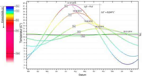
The amplitudes of the sinsoidal temperature gradients clearly decline with increasing soil depth. Simultaneously, a phase shift takes place so that external air temperature peaks reach the deeper regions much later on. The amplitude peaks of 21.5 °C (on 21.07) in the test reference years shown here only has an impact 91 days later at a depth of 5 m. Here the peak temperature was still 13.1 °C on 20.10. With increasing depth, an almost constant temperature at the level of the mean annual temperature is reached. The high phase shifts no longer allow a purely steady-state consideration of the transmission heat losses for the monthly method since the charging and discharging processes may extend over several months. Heat storage in the ground and the resultant damping action and phase shifting of the ground temperature under the floor slab is therefore of significance when calculating heat losses through the ground.

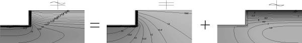
In the PHPP this problem is analysed using the principle of superposition. The sinusoidal gradient of the heat flow is divided into a steady-state $L_s$ and a harmonic component $L_{pe}$. Both parts can be adjusted in the PHPP by means of a linear thermal transmittance. In contrast with $L_s$, $L_{pe}$ must be adjusted using a harmonic linear thermal transmittance which should be determined by means of a transient state simulation; however, for simplification this can also be equated with the steady-state Ψ-value.

This video clip shows the temperature profile under floor slab of a building for three different cases:

1. simple floor insulation, i.e. floor slab with thermal insulation underneath
2. skirt insulation, i.e. floor slab without insulation, but with a strip of insulation all around the building,
3. without insulation

The temporal course of the heat loss through the three floor slab types is shown in parallel.

Further literature on the topic of skirt insulation:

[AkkP 48] Using Passive House technology for retrofitting non-residential buildings/ Heat losses towards the ground ; Protocol Volume No. 48 of the Research Group for Cost-effective Passive Houses, 1st Edition, Passive House Institute, Darmstadt 2012 (Link zur Publikationsliste des PHI)

For calculating thermal bridges in the area in contact with the ground, a steady-state approximation suffices in many cases and dynamic simulation can be dispensed with. Although dynamic simulations provide more accurate results, they also incur additional effort. Moreover, on account of the usually only imprecisely known thermal characteristics of the ground, the expected accuracy of a one-dimensional or two-dimensional transient numerical calculation is not so high that this extra effort can also be justified (except in the case of large or research projects). Frequently, the Ψ-values calculated in a steady-state manner are therefore also used as harmonic Ψ-values (see the Ground worksheet in the PHPP). However, for thermal bridges of areas in contact with the ground which are far away from the ground surface, this assumption is will usually be quite pessimistic. Whether it is worthwhile to perform a time-dependent calculation is easily determined by setting the harmonic Ψ-value in the PHPP to the same value as the steady-state Ψ-value one time, and equal to zero another time and then observing the influence on the final result. A steady-state calculation under the mentioned boundary conditions can also give pessimistic results with respect to the surface temperatures.

[AkkP 27] Heat losses through the ground; Protocol Volume No. 27 of the Research Group for Cost-effective Passive Houses,
1st Edition, Passive House Institute, Darmstadt 2004 (Link to list of PHI publications)

• Basic principle for calculating thermal bridges
• Recommended procedure for calculating thermal bridges of components in contact with the ground
• Examples of thermal bridge calculations